The cellular slime mould Dictyostelium discoideum is a soil protozoan that feeds on bacteria. This model organism has been extensively studied, as the life cycle of the organism provides a unique opportunity to study the relation between signal transduction at the cellular level and morphogenesis and behaviour at the multicellular level. Upon starvation, individual amoebae aggregate and form migrating multicellular slugs. During aggregation the amoebae differentiate into prestalk and prespore cells. The prestalk cells group into the front part, while the rear part consists of prespore cells. Each slug culminates in a fruiting body consisting of a globule of spore cells on a slender stalk.
The aggregation is orchestrated by waves of cAMP, which are formed by a combination of a pulsatile cAMP excretion and a cAMP-mediated cAMP response; the amoebae show a chemotactic response towards cAMP. This combination of waves of excitation and chemotaxis persists during the slug stage.
Migrating slugs are orientated by temperature gradients. This thermotaxis shows a significant temperature adaptation, with positive thermotaxis at temperatures above the temperature during aggregation, and negative thermotaxis below this temperature (Whitaker & Poff, 1980). At night, the soil surface is cooler than the subsurface mulch, and hence the slug is directed by negative thermotaxis towards the surface. At daytime the reverse is true, but the slug still moves upwards, this time due to positive thermotaxis. As a result, the slug always tends to migrate towards the soil surface where it will fruit, thus ensuring good conditions for spore dispersal (Bonner et al., 1985).
How a temperature gradient is converted into tactic behaviour is not yet fully understood, but several researchers have shown that ammonia (NH3) plays an important role in this process, since temperature influences NH3 production significantly, and thermotaxis diminishes when slugs are surrounded by NH3 (Bonner et al., 1989). Three roles of NH3 have been proposed. First, thermotaxis may be due to negative chemotaxis away from NH3. Several authors have reported such negative chemotaxis, and have shown that a slug can produce sufficient concentrations of NH3 to account for such an orientation (Feit & Sollitto, 1987; Yumura et al., 1992; Bonner et al., 1986; Kosugi & Inouye, 1989).
A second role of NH3 may be that it speeds up cell motion. Bonner et al. (1986) reported such an increase of cell motion due to NH3. Based on this result, a model was constructed for thermotaxis (Bonner et al., 1989). However, this report is still disputed. van Duijn & Inouye (1991) found that NH3 only slightly, non-significantly, increased the chemotactic-locomotion speed. In fact, more detailed studies reported that average slug speed may be unaffected by NH3 or temperature gradients (Fisher, 1997; Smith et al., 1982). Furthermore, Davies et al. (1993) reported that NH3 did not cause any change in the chemotaxis towards cAMP.
Thirdly, NH3 may affect the cAMP signalling. Schindler & Sussman (1979) showed that NH3 inhibits the cAMP-induced cAMP release. The underlying mechanism is that NH3 blocks the intracellular cAMP accumulation, due to the inhibition of the transitory activation of adenylate cyclase in response to the binding of extracellular cAMP to cell surface receptors (Davies et al., 1993; Williams et al., 1984). Furthermore, Darcy & Fisher (1990) produced evidence that this inhibition of the cAMP signalling is important in slug behaviour.
We use only the latter role of NH3 in our model. As a shortcut, we model the inhibition of the cAMP relay by NH3 as a direct (negative) influence of temperature on the excitability.
There have been several models describing slug migration (Bretschneider et al., 1995; Williams et al., 1986; Savill & Hogeweg, 1997; Dormann et al., 1998; Umeda, 1989; Odell & Bonner, 1986). However, until now no one has used a model for slug migration to describe thermotaxis. The purpose of this study, therefore, was to determine whether thermotaxis can be achieved using basic and accepted principles of Dictyostelium information processing at the cellular level. To study this topic, we used the model of Savill & Hogeweg (1997) because it handles pressure, deformation, and motion in a very elegant way, and enables us to investigate thermotaxis in the context of the complete development from single cells to fruiting bodies. The model of Savill & Hogeweg is three-dimensional (3D), but for our purposes we can use two-dimensional (2D) simulations. Besides, very recently Bonner (1998) presented a new method in which migrating 2D (one cell thick) slugs are produced at a glass-mineral oil interface. This creates the opportunity to compare our results directly with the experimental findings of Bonner.
In our model, thermotaxis is achieved by a modification of the cAMP waves, due to the differences in the excitability. These differences change the shape of the wave, and chemotaxis towards the wave leads to the tactic behaviour.
We have used the hybrid CA/PDE model of Savill & Hogeweg (1997), which is based on the CA model of Glazier & Graner (1993). In this model, a CA is used to represent individual amoebae, and a PDE to model the cAMP dynamics. An important feature of the model is that each amoeba is represented as a group of connected automata. As a consequence, amoebae can slide past one another and deform themselves and adjoining amoebae by means of small changes in their boundaries.
The space where the slug crawls is a 2D lattice. Each lattice square
represents an automaton as well as a grid point in the numerical PDE.
Each amoeba has a unique identification number, ![]() , which is
assigned to all automata which form the amoeba.
, which is
assigned to all automata which form the amoeba. ![]() = 0 represents
the medium. Amoebae have also a label
= 0 represents
the medium. Amoebae have also a label ![]() , which indicates whether
their cell type is prespore, prestalk or autocycling prestalk
(
, which indicates whether
their cell type is prespore, prestalk or autocycling prestalk
(![]()
![]() {p, t, a}).
{p, t, a}).
Each automaton that is part of an amoeba's boundary, i.e. for which one
of its eight neighbouring automata does not belong to the same amoeba,
has dimensionless free energy bonds. The magnitude of these bonds
depends on the cell types they connect. The energy bonds are given by
J![]() ,
,![]() > 0, where
> 0, where ![]() are the types of the
adjoining amoebae. The bond energy between an amoeba and the medium is
given by
J
are the types of the
adjoining amoebae. The bond energy between an amoeba and the medium is
given by
J![]() , M. The total free energy of an amoeba is given by:
, M. The total free energy of an amoeba is given by:
In order to model an amoeba deforming its shape, we use the following
rule: an automaton is chosen at random and the state of one of its
neighbours is copied into it with a probability of occurring given by:
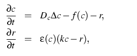
The cAMP signalling system is rather complex and can be described using detailed models, such as, e.g. Martiel & Goldbeter (1987) and Tang & Othmer (1994). However, the dynamics can be described reasonably well in a quantitative way by two variable simplified equations of the FitzHugh-Nagumo (FHN) type (see e.g. Grindrod, 1996). Such a description reproduces the overall characteristics of cAMP waves such as refractoriness, eikonal-curvature relation, etc. The main advantage of these models is their simplicity and therefore their capacity to connect the effects visible in these models with basic properties of the cAMP signalling in Dictyostelium.
Here we investigate the basic effects of heterogeneity in the
excitability, but we are not concerned with the details of cAMP
signalling. So for our present purposes, the FHN-models are preferred.
In this paper, we use FHN-type equations with piecewise linear
`Pushchino kinetics' (Panfilov & Pertsov, 1984). This system allows for
even greater control of the refractory periods and is much faster to
compute than the classical system (Panfilov, 1991):
Weijer et al. (1984) showed that the tip of the slug can be seen as a
high-frequency pacemaker, whereas the body of the slug just conducts
waves of cAMP. We can model this in the following way. For positive
values of parameter a![]() , the model describes an excitable medium,
while for negative values of a
, the model describes an excitable medium,
while for negative values of a![]() , a stable limit cycle appears in
phase space. Therefore, to describe the excitable amoebae, we have
chosen
ap = at = 0.1, whereas to describe the autocycling amoebae in
the tip, aa = - 0.1.
, a stable limit cycle appears in
phase space. Therefore, to describe the excitable amoebae, we have
chosen
ap = at = 0.1, whereas to describe the autocycling amoebae in
the tip, aa = - 0.1.
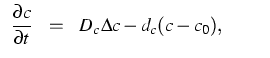
To illustrate these basic properties of the model, we plot in
Fig. 3.1 the phase plane of c and
r. Figure 3.1(a) shows the situation when
a![]() = - 0.1. The nullclines intersect at an unstable equilibrium
point, and the dynamics show a stable limit cycle. The inset shows the
oscillatory behaviour in time. Figure 3.1(b) shows
the phase plane when
a
= - 0.1. The nullclines intersect at an unstable equilibrium
point, and the dynamics show a stable limit cycle. The inset shows the
oscillatory behaviour in time. Figure 3.1(b) shows
the phase plane when
a![]() = 0.1. Now the equilibrium point is
stable, and the system relays a cAMP signal if the initial
concentration of cAMP exceeds the threshold value.
= 0.1. Now the equilibrium point is
stable, and the system relays a cAMP signal if the initial
concentration of cAMP exceeds the threshold value.
 |
We simplify the whole process of differential NH3 production due
to the temperature gradient, followed by differential inhibition of
the cAMP-modulated cAMP response due to NH3, by stating that the
temperature gradient causes a spatial gradient in the excitability. We
have chosen to model the differences in the excitability by changing
the value of a![]() , since in this model a
, since in this model a![]() represents the
threshold for cAMP relay, which is directly related to the
excitability. We superimpose on the values of a
represents the
threshold for cAMP relay, which is directly related to the
excitability. We superimpose on the values of a![]() a gradient
along the y-axis, with a slope of
agrad per grid
point, and with decreasing excitability from top to bottom. We
normalise the gradient by taking the upmost automaton that is occupied
by the slug as the reference point to calculate all a
a gradient
along the y-axis, with a slope of
agrad per grid
point, and with decreasing excitability from top to bottom. We
normalise the gradient by taking the upmost automaton that is occupied
by the slug as the reference point to calculate all a![]() values. We use a normalised gradient to assure that the behaviour is
independent of the location of the slug in the field.
values. We use a normalised gradient to assure that the behaviour is
independent of the location of the slug in the field.
The natural way to incorporate chemotaxis in the model is to use the
spatial gradient of the cAMP wavefront. We do this by modifying the
change in energy ![]() H in eqn (3.2), and hence the
probability of the neighbour copying its state into the automaton, as
a function of the difference in the cAMP concentrations in the two
automata (Savill & Hogeweg, 1997):
H in eqn (3.2), and hence the
probability of the neighbour copying its state into the automaton, as
a function of the difference in the cAMP concentrations in the two
automata (Savill & Hogeweg, 1997):
In all simulations a slug is initiated with a tip consisting of autocycling prestalk cells, and a body consisting of 40% prestalk and 60% prespore cells.
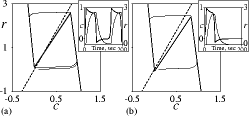
Figure 3.2(a) shows slug motion in a simulation without thermotaxis. Repeatedly the chemotactic signal spreads from the autocycling cells in the tip towards the posterior part of the slug. The subsequent chemotactic motion pushes the tip forwards, and as a result the whole slug moves ahead. We see that the slug does not follow a straight line. Its trail shows alterations in direction, caused by small variations in the way the tip is pushed forwards.
 |
As can be seen in Fig. 3.2, during the simulations, which take up 300,000 time steps (8 hours and 20 minutes), the shape of the slug is approximately fixed. This stable configuration results from two forces; one elongates the slug, and the other one rounds it. The surface tension forces the slug to round, since this is the optimal low-energy configuration, whereas the convex-shaped cAMP wave causes a motion of the amoebae towards the central axis, and therefore forces the slug to elongate.
Different surface tensions lead to different slug shapes. Hence we
chose the values of
J![]() , M so that the surface tension between
the cell types and the medium, which is defined by
Glazier & Graner (1993) as
J
, M so that the surface tension between
the cell types and the medium, which is defined by
Glazier & Graner (1993) as
J![]() , M -
, M - ![]() J
J![]() ,
,![]() , is
equal for all cell types.
, is
equal for all cell types.
The convex shape of the cAMP wave is caused by two factors: first, every new cAMP wave originates as a circular wave from a point source, which immediately leads to a convex wave shape. Secondly, the speed of the cAMP wave is lower at the slug boundary, because amoebae along the boundary of the slug are less excitable, due to loss of cAMP into the surrounding medium.
In our computations we have chosen an initial shape which is close to the final shape of the slug. By starting with another shape, which is thinner or thicker than the optimal shape, one adds extra transient behaviour, but the final configuration is the same.
Figure 3.3 shows the relation between the slug
mass and the motion velocity. To measure motion velocity, tracks of
slugs were followed during
5![]() hours (200,000 time
steps). We see that if a slug consists of 20 amoebae, velocity is only
50% of the maximum velocity, while larger slugs clearly move
faster. This increase in motion velocity seems to saturate when the
number of amoebae gets close to 1000. Our results are consistent
with the experimental data: it is known from experiments that the slug
velocity increases with increase in the slug size
(Smith et al., 1982; Bonner et al., 1953), and
Inouye & Takeuchi (1979) showed the saturation of velocity increase for
large slugs.
hours (200,000 time
steps). We see that if a slug consists of 20 amoebae, velocity is only
50% of the maximum velocity, while larger slugs clearly move
faster. This increase in motion velocity seems to saturate when the
number of amoebae gets close to 1000. Our results are consistent
with the experimental data: it is known from experiments that the slug
velocity increases with increase in the slug size
(Smith et al., 1982; Bonner et al., 1953), and
Inouye & Takeuchi (1979) showed the saturation of velocity increase for
large slugs.
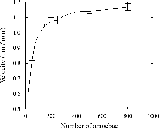 |
The velocity increase we found is on the one hand due to the fact that more amoebae create more motive force to push the autocycling area forwards, since this region does not create a motive force by itself. On the other hand, to the fact that the motive force created by the slug does not solely depend on chemotaxis towards cAMP. Also the accompanying volume changes, and the binding strengths as well as the surface tension play an important role: First, due to the binding forces between the amoebae, amoebae start moving before the cAMP wave arrives, as they are pulled towards the chemotactically moving amoebae. Secondly, the surface tension creates a forward motion to fill up the dents in the slug shape just posterior of the cAMP wave. Thirdly, due to volume decrease during the chemotactic motion, as many cells push inwards, motion lasts after the cAMP wave has passed, to re-establish the old volume. Since all these depend on the slug size, the motion is faster when the slug is larger.
The saturation in volume increase with size, as described by Inouye & Takeuchi (1979), occurs in slugs with much larger number of amoebae than in our finding. This can be caused by the fact that we performed 2D simulations, and can be due to scaling reasons.
It has been known for some time that cell sorting takes place mainly during the mound stage that precedes the slug stage. However, both dissociation experiments (Sternfeld & David, 1981) and transplantation experiments (MacWilliams, 1982) have shown that slugs are still fully capable of exhibiting cell sorting.
In our simulations we start from a random distribution of prestalk and
prespore cells, and after 4 hours prestalk and prespore cells are
completely sorted out. In our model, this cell sorting is solely due to
differential adhesion, since there are no other differences between
the cell types. When
J![]() ,
,![]() is smaller, amoebae with the same
inelasticity
is smaller, amoebae with the same
inelasticity ![]() deform less, since the final term in
eqn (3.1), which ensures volume conservation, is relatively
more important. As a consequence, the extra motive force of pulling
the cells forwards is larger. In contrast, when
J
deform less, since the final term in
eqn (3.1), which ensures volume conservation, is relatively
more important. As a consequence, the extra motive force of pulling
the cells forwards is larger. In contrast, when
J![]() ,
,![]() is
larger, the amoebae just deform and hence have a relatively slower
motive speed. Thus, to obtain autocycling cells in the tip, followed
by prestalk cells, and finally prespore cells,
Ja, a < Jt, t < Jp, p. The binding energies between the cell types are less
important for cell sorting. They are kept high enough to assure that
the cell types do not mix, and are kept low enough to assure that
amoebae of different cell types are still able to slide past one
another, which is necessary for large-scale cell sorting.
is
larger, the amoebae just deform and hence have a relatively slower
motive speed. Thus, to obtain autocycling cells in the tip, followed
by prestalk cells, and finally prespore cells,
Ja, a < Jt, t < Jp, p. The binding energies between the cell types are less
important for cell sorting. They are kept high enough to assure that
the cell types do not mix, and are kept low enough to assure that
amoebae of different cell types are still able to slide past one
another, which is necessary for large-scale cell sorting.
In our simulations, if a clump of autocycling cells are positioned closely behind the tip, these cells become entrained to the cAMP signalling from the tip, and moreover, after some time, by the process of cell sorting as described above, the clump reunites with the autocycling cells in the tip (results not shown). Only if either the clump or the difference in the excitability with the surrounding cells is large enough, these cells themselves become a new source of cAMP signalling, which, after some time, results in the break up of the slug into two small ones.
We were able to reproduce thermotaxis of the Dictyostelium slug. Figure 3.2(b) shows slug motion in a field with a temperature gradient directed from top to bottom. Initially the slug is orientated at an angle of 90 degrees to the direction of the gradient. Yet within 3 hours the slug orientates itself towards the gradient.
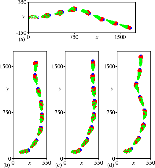
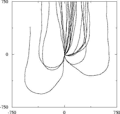
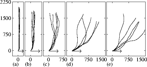
Figure 3.4 shows the tracks of Dictyostelium slugs from 25 different simulations, with initial angles of 0, 45, 90, 135, and 180 degrees to the temperature gradient. It can be seen that the final direction of motion does not depend on the initial angle. Even if the initial angle is 180 degrees, standard irregularities in the track cause small deviations in the angle that are large enough to elicit the subsequent turn, either to the left or to the right.
 |
In our model, we assume a temperature dependence of the cAMP-induced
cAMP release (presumably mediated by NH3). We implement this as a
change in the excitability, i.e. by a modification of the value of
the a![]() parameter. Hence, we change the cAMP threshold. An
increased threshold changes both the period of autocycling and the
velocity of the cAMP wave. Figure 3.5(a) shows the
dependence of the period on a in the oscillatory regime, i.e. for
negative values of a. Figure 3.5(b) shows the
dependence of the velocity on a in the excitable regime, i.e. for
positive values of a (note that in the oscillatory regime wave
velocity depends on both period and relay). For reasonable values of
a the period increases with increasing a, and over the whole range
of values the velocity decreases. Both are important for the mechanism
of thermotaxis as they influence both the source of the cAMP signal
and the shape of the cAMP wave.
parameter. Hence, we change the cAMP threshold. An
increased threshold changes both the period of autocycling and the
velocity of the cAMP wave. Figure 3.5(a) shows the
dependence of the period on a in the oscillatory regime, i.e. for
negative values of a. Figure 3.5(b) shows the
dependence of the velocity on a in the excitable regime, i.e. for
positive values of a (note that in the oscillatory regime wave
velocity depends on both period and relay). For reasonable values of
a the period increases with increasing a, and over the whole range
of values the velocity decreases. Both are important for the mechanism
of thermotaxis as they influence both the source of the cAMP signal
and the shape of the cAMP wave.
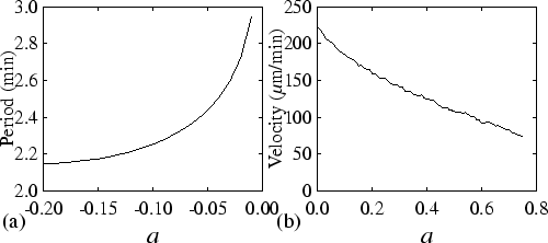 |
Figure 3.6 shows a close up of the cAMP wave. Figure 3.6(a) shows the cAMP wave during normal motion, while Fig. 3.6(b) shows the wave during thermotaxis. To emphasise the effect of the temperature gradient on the shape of the cAMP wave, we have chosen a rather high value of agrad = 2.5×10⁻³. During thermotaxis, the source of the signal in the autocycling area shifts upwards, since in the upper direction a values are lower, and subsequently the autocycling period is shorter. Besides, as a result of the dependence of wave speed on a, the wave moves faster at the upper side compared to the lower side. As a consequence of both, the wavefront becomes slanted. However, the slant increases only up to a certain level, since it coincides with a curvature difference that limits the slant, due to the so-called curvature-effect.
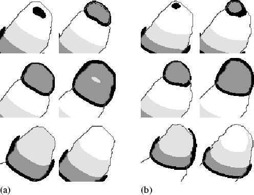 |
Since the amoebae move perpendicular to the wavefront, a motive force is created that pushes the autocycling area upwards, and with it the source of the cAMP signal, thus initiating the turn towards the temperature gradient.
We studied thermosensitivity as a function of agrad. Figure 3.7 shows the tracks of slugs from simulations with different gradient strengths. In all simulations, the initial angle is 90 degrees to the temperature gradient. In Fig. 3.7(a) and (b), we see that when the gradient is very steep, the slugs show a rapid turn towards the temperature gradient. After this turn, the track is very stable and perfectly aligned along the temperature gradient. In Fig. 3.7(c) and (d), we see that when the gradient becomes more shallow, turning of the model slug takes increasingly more time, and the final track becomes more and more unstable. In Fig. 3.7(e) the gradient is as small as agrad = 1.5×10⁻⁴. Although the slugs do not move along the temperature gradient, they still move in the right direction. Note that we even found thermosensitivity for much smaller agrad, i.e. agrad = 6×10⁻⁵.
 |
However, in an environment with such shallow gradients, one expects to
find a relatively high level of disturbance on the signal. Besides,
there must exist some variation in the excitability between individual
amoebae. Therefore, an important question is whether an addition of
noise to the values of a![]() reduces or diminishes thermotaxis.
reduces or diminishes thermotaxis.
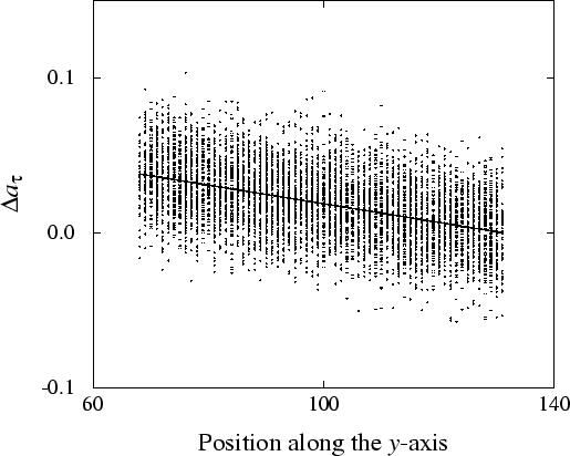
To test the sensitivity to disturbances, spatiotemporal Gaussian
noise is added to the value of a![]() , with a refreshment rate of
2 seconds (20 time steps). We expect that in real slugs disturbances
are high, relative to the shallow gradients at which a Dictyostelium slug still
exhibits thermotaxis. Therefore we use a high noise term, with a
normal distribution of mean=0, and S.D.=0.02,
i.e. which is more than 30 times as large as
agrad. Figure 3.8 gives an impression
of the signal to noise ratio for a certain moment in time. The
ordinate denotes the location of the slug in the y-direction, the
abscissa gives the corresponding increase of a
, with a refreshment rate of
2 seconds (20 time steps). We expect that in real slugs disturbances
are high, relative to the shallow gradients at which a Dictyostelium slug still
exhibits thermotaxis. Therefore we use a high noise term, with a
normal distribution of mean=0, and S.D.=0.02,
i.e. which is more than 30 times as large as
agrad. Figure 3.8 gives an impression
of the signal to noise ratio for a certain moment in time. The
ordinate denotes the location of the slug in the y-direction, the
abscissa gives the corresponding increase of a![]() . The solid
line shows the gradient in the absence of noise. The dots show the
increase of a
. The solid
line shows the gradient in the absence of noise. The dots show the
increase of a![]() for all individual automata in the presence of
noise. Note that the gradient is very difficult to detect when noise
is present. Figure 3.2(c) shows a simulation with
this spatiotemporal noise. In spite of the high level of noise, both
precision and turning velocity are not decreased. In fact, noise
levels have to be increased more than ten times before thermotaxis
diminishes.
for all individual automata in the presence of
noise. Note that the gradient is very difficult to detect when noise
is present. Figure 3.2(c) shows a simulation with
this spatiotemporal noise. In spite of the high level of noise, both
precision and turning velocity are not decreased. In fact, noise
levels have to be increased more than ten times before thermotaxis
diminishes.
 |
Secondly, we create heterogeneity in the amoebae population. The same level of variation is used as in the previous simulation, but this time only one noise value is used for all grid points which are part of the same amoeba. This value is fixed during the whole simulation. Figure 3.2(d) shows such a simulation. Although the track is less stable compared to simulation 3.2(c), thermotaxis is still strong. Noise levels can be increased up to 60 times the gradient strength, but at higher values of the noise S.D., different sources of cAMP waves appear, which break the slug into an increasingly higher number of ever smaller slugs.
The mechanism behind this high resistance against noise is that the cAMP wave functions as a spatiotemporal integrator. Due to the curvature-effect, the cAMP wavefront is always a relatively smooth line. Differences in position are found only over longer distances. Consequently, the shape, as observed, results from the information integrated over longer time and larger distances. And since it is the chemotaxis towards this wave that gives rise to the thermotactic behaviour, global information integration becomes possible. The same process makes it possible to measure extremely small gradients, despite some internal noise generated by the model itself.
In the second experiment, with variation at the level of the individual amoebae, the variations are both temporally and spatially on a larger scale. Therefore, thermotaxis is more disturbed by this kind of noise.
Several researchers have stated that the process of orientation is located in the slug tip (Fisher, 1997; Smith et al., 1982). This could either indicate that there is an inherent difference between the different cell types, for example that only autocycling amoebae in the tip are thermosensitive, or that there is a functional difference between parts of the slug, i.e. all amoebae share the same thermosensitivity, but differ in behaviour solely due to their relative position inside the slug.
Figure 3.9 shows the velocity at which slugs turn towards the temperature gradient. The turning velocity is calculated using data from 10 simulations per line, taking into account the symmetry left and right of the direction of the gradient. The figure shows the differences in the turning velocity, whether or not the tip or the rest of the slug is thermosensitive.
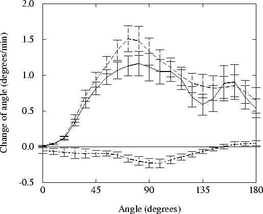 |
If the slug tip is not thermosensitive, indeed no thermotaxis whatsoever can be observed. On the other hand, desensitising the rest of the slug has no negative effect on thermotaxis. For certain angles the turning velocity is even slightly higher. Still, both when the whole slug is thermosensitive and when only the tip is thermosensitive, slugs turn with approximately the same velocity and the same precision towards the temperature gradient.
We have shown that our model can reproduce important features and processes which occur in the slug, such as slug motion, cell sorting, shape conservation and the dependence of slug velocity on its mass.
In the model we have developed, the motive force is obtained by a combination of chemotaxis towards cAMP and cell adhesion (see also Savill & Hogeweg, 1997). Instead, Williams et al. (1986) suggested that circumferential cells may squeeze and push forwards the inner cell mass, while Odell & Bonner (1986) suggested that this may be achieved by a fountain-like circulation of cells. However, fluorescence images indicated neither the circumferential movement of cells toward the inner cell mass nor active movement backwards (Yumura et al., 1992).
Siegert & Weijer (1992) showed that 3D scroll waves organise the tip. Based on these results, Bretschneider et al. (1995) made a model to describe slug motion directed by scroll waves, which is essentially the same mechanism as we use. For reasons of simplicity, we did only simulations in 2D, and therefore, such waves were not possible in our simulations. However, behind the tip the scroll wave rapidly breaks up into planar waves, due to decreasing excitability (Dormann et al., 1996). We state that in our model we focused on these planar waves. Obviously, 3D simulations will extensively enlarge the set of possible behaviours, but the recent experiments of Bonner (1998) show that all observations of 2D slugs are consistent with what one finds in normal 3D slugs.
In all our simulations, we used a tip consisting of oscillatory amoebae, while the rest of the slug only relayed the signal. However, the change in the excitability might be much more gradual, with many more cells being in the oscillatory regime (Dormann et al., 1996; Siegert & Weijer, 1992). Therefore we performed a number of control experiments, in which all cells were oscillatory, although the tip cells were still the most excitable ones ( at = ap = - 0.05). All other conditions were kept the same. This caused no qualitative differences in any model behaviour: the high-frequency oscillations in the tip still enforce the global cAMP dynamics.
In order to obtain a stable shape of the slug, in our model, it is necessary to have a convex wave shape, which is caused by the reduced relay at the slug boundaries. In real slugs this can be a consequence of the fact that migrating slugs are covered with slime sheath, a viscous extracellular matrix secreted by its cells. We have not explicitly modelled the slime sheath, but we interpret the diffusive loss of cAMP as being due to diffusion into this sheath. However, if we use Neumann boundary conditions, which means that there is no flux of cAMP through the boundary and hence no reduced relay, all other behaviour, such as slug motion, cell sorting and thermotaxis, are still preserved. That is, only the shape becomes inconsistent.
During the slug stage, cell redifferentiation still occurs, but it is likely to be a marginal and slow process (Schaap et al., 1996), and was left out of the model. Instead we focused on cell sorting. In our simulations, we used 40% prestalk cells, while a more realistic value is around 25%. Reducing the percentage of prestalk cells in our computations to 25% does not significantly change the results of our paper: complete cell sorting is still observed, although on a slightly longer time-scale. Hence, to present both thermotactic behaviour and cell sorting in the same time sequence, we increased the number of prestalk cells used. Cell sorting with a small amount of prestalk cells is slow due to the formation of very small clumps of prestalk cells. This is mainly a side-effect of our 2D approach, since in 3D larger clumps are immediately formed, as a result of the higher amount of neighbouring amoebae (Savill & Hogeweg, 1997).
Umeda (1989) proposed a model for cell sorting, based on differential motive forces, and Bretschneider et al. (1997) also used differential chemotaxis to model sorting. However, Sternfeld (1979) found evidence that the cell sorting depends on differential cellular adhesion, and recently, Ginger et al. (1998) have found a cell surface protein which is important for both cell adhesion and cell sorting.
Sternfeld & David (1981) found that during the process of cell sorting, cAMP is also very important. In our model, the cell sorting takes place during the cell motions that accompany the cAMP waves. We find very slow and incomplete cell sorting when we do not include the chemotactic motion towards cAMP. This is in agreement with the above finding, as well as with the results of Tasaka & Takeuchi (1981), which show that cell sorting is facilitated by the movement of the amoebae.
MacWilliams (1982) and Meinhardt (1983) found that injecting prestalk cells into the rear part of a slug leads either to a movement of these cells towards the tip, or to the induction of a new tip, followed by the separation of a second slug. This is also in agreement with our results as described in section 3.3.3.
Bonner (1998) found that the amoebae in the tip of 2D slugs move around in a chaotic fashion, while the posterior cells move straight on. In our model, we find the same behaviour: in the tip all amoebae try to move towards the source of the cAMP signal, thereby creating chaotic and swirling motion. Behind the tip the closed cAMP wave leads to straight motion.
In our model, motion is far more continuous, compared to the pulsatile cAMP signal, due to the pushing and pulling at large distances from the wavefront. The small 2D slugs that Bonner (1998) has described, do also not exhibit sharp pulsatile motion.
We have shown that thermotaxis of Dictyostelium slugs can be explained solely by means of a temperature dependence of the cAMP-induced cAMP release and the consequences thereof for the excitability. It changes the shape of the cAMP wave, and chemotaxis towards the wave leads to the tactic behaviour: independent of the initial orientation, the slug turns towards and, afterwards, moves along the temperature gradient. The slug has a very high sensitivity, since even in the presence of extreme noise in the system (the signal-to-noise ratio can be as small as 1/300), it receives the temperature signal.
The slug behaviour in our model is due to the collective behaviour of the amoebae, as the temperature gradient is too shallow to be measured by individual amoebae. Instead, the information is first encoded as differences in the excitability.
The aim of this study was to describe the basic processes which can give rise to thermotactic behaviour. We have not modelled the translation of differences in temperature into differences in excitability. We assume that this process involves chemicals such as NH3, and maybe several other chemicals, such as Slug Turning Factor (STF) (Fisher, 1997). In our paper, we have used a linear gradient which we normalised within the slug. In our view, such normalisation is a good approximation of slug behaviour at a short time-scale. However, at longer time-scales, the relation between temperature and excitability is clearly more complicated, since both positive and negative thermotaxis are observed, as well as slow adaptations to the absolute temperature (Whitaker & Poff, 1980). For very shallow gradients, we do not need adaptive processes (in our implementation: normalisation of the gradient) in our model, for excitability can be coupled directly to the absolute temperature. However, to describe larger temperature differences an adaptive process is necessary. Instead of the normalisation used here, the model could be extended with an extra equation for a, depending on temperature, which describes the differences in the excitability at a fast time-scale, as well as a return to the basal level at a slow time-scale. With such an extension, one could model the negative thermotaxis as well as the adaptation and compare both with observed experimental behaviour.
There has been a fair amount of dispute whether NH3 speeds up the amoebae. Therefore, we did not include an increase in velocity due to NH3 in our model. We do not state that amoebae under no conditions will have such a stronger motive force, but we show that it is not a necessary condition for thermotaxis: if there are differences in NH3, which change excitability only, thermotaxis can already be found.
Recently, Bonner (1998) has concluded that his idea of differences in the speed of motion to explain thermotaxis is not consistent with what one sees in 2D slugs. Instead, he observes that many different and changing cells are involved in pushing the tip into a different direction, which is exactly in agreement with our results.
In our model, it is mainly the tip that controls the orientation, which is in agreement with experimental findings. However, continuous cell sorting and differentiation during the slug motion, which is accompanied by ongoing changes in position, makes it unlikely that only the tip is thermosensitive, since it is observed that such a special property is not needed for thermotaxis.
A very high number of genes are in one way or another related to thermotaxis (Fisher, 1997). We did not aim to include in our model all that is known, but instead we focused on the question which types of behaviour can be understood from some basic principles of signal transduction in Dictyostelium. In this light, the function of all these genes might be interpreted as the tuning of the parameters to get the favoured behaviour.
This method of cell modelling lends itself excellently for describing the morphogenesis of Dictyostelium discoideum, since the different behaviours observed during the developmental process are entirely driven by the local movements and responses of individual amoebae. It was used earlier to describe the process of aggregation, mount formation and slug motion (Savill & Hogeweg, 1997), and is used here to describe a range of observed behaviours during the slug stage. By extending the model once again to 3D, the next stages of development, as well as other facets of Dictyostelium morphology, may be clarified.
 +
+